How to Score Economic Security

Chokepoints, surge capacity, and accountability

Earlier this year we launched an economic security contest. We had two prompts:

• What are the most important high level KPIs that policy should aim for? What is the analogy of the Fed’s ‘2% inflation and full employment’ target for economic security?

• Where today would you put $10-50bn to get the most for your investment in economic security? Feel free to propose both defensive and offensive ideas, and either a portfolio of ideas or the one large idea you think will deliver the most value.

Last week we ran our first essay winner.

Our second essay comes from Naveen Krishnan, a Belfer Young Leaders research fellow at Harvard with the Belfer Center for Science and International Affairs, where he specializes in artificial intelligence capabilities and U.S. national security policy. He is an intelligence officer in the U.S. Navy Reserve. His views are his own and do not represent those of the U.S. Navy or Harvard.

---

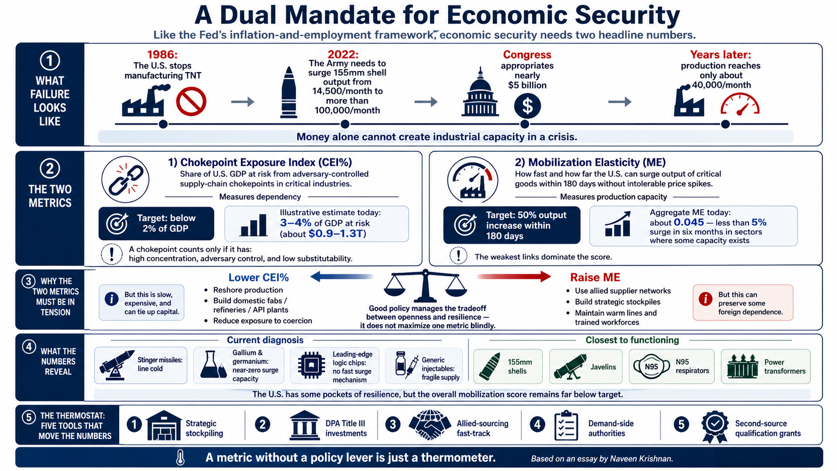
The United States stopped manufacturing its own TNT in 1986. For decades afterward, the Army bought its primary explosive fill from Russia and Ukraine. When one supplier invaded the other in February 2022, the Army needed to surge 155mm artillery shell production from 14,500 rounds per month to over 100,000. The binding constraint (instead of money) was America’s physical inability to produce the explosives, propellants, and shell casings at the required pace. Congress appropriated nearly $5 billion. But four years and billions of dollars later, production has reached only 40,000 rounds per month.

This is what an economic security failure looks like: the absence of the industrial base required to turn money into output under crisis conditions - regardless of how ‘urgently’ Congress pushes. Money is not a magic wand for manufacturing; in a crisis, you cannot simply legislate or spend your way out of the physical reality of industrial systems. The U.S. remains vulnerable precisely when surges are necessary: a scenario where we have the capital to buy, but no physical mechanism to produce.

Across the political spectrum, policymakers recognize this crisis and see that the U.S. government must take a more active role in securing the supply chains that underpin national power. Yet this activism lacks a dashboard. We have no headline numbers that tell policymakers whether the United States is becoming more secure or less secure, by how much, and where the gaps are. Policy debates fruitlessly devolve into competing lists of vulnerabilities (e.g. chips, minerals, pharma) without a unifying framework for tradeoffs. The result is incoherent allocation: billions for flagship semiconductor fabs while the Army cannot produce enough artillery shells for a single theater war.

This essay proposes the missing headline: two metrics, in productive tension, that together define economic security the way inflation and unemployment define macroeconomic health for the Federal Reserve.

A Dual Mandate for Economic Security: The Chokepoint Exposure Index and Mobilization Elasticity

Metric 1: Chokepoint Exposure Index (CEI%): The percentage of U.S. GDP at risk from adversary-controlled supply chain chokepoints across critical industries. This measures dependency: where the economy is vulnerable to coercion. Target: below 2% of GDP.

Metric 2: Mobilization Elasticity (ME): The speed and scale at which the U.S. can surge production of critical goods (e.g. finished weapons systems, essential medicines) under crisis conditions, without destabilizing or intolerable price spikes. This measures production capacity: whether the economy can actually respond when coercion hits. Target: 50% output increase within 180 days.

The first metric tells policymakers where the economy is exposed. The second tells them whether it can fight back. Together, they force the tradeoffs that matter most: engagement versus self-sufficiency and openness versus resilience: the central balancing acts of economic security in the age of weaponized interdependence.

The Productive Tension

The Fed’s dual mandate (maximize employment, stabilize prices) works as a policy framework precisely because its two targets pull against each other. Pushing unemployment down requires stimulative policy (low interest rates, quantitative easing) that risks overheating prices. Pushing inflation down requires restrictive policy (high interest rates, tighter credit) that risks killing jobs. The tension is the point: it forces the Fed to find the frontier between the two goals rather than blindly maximizing one at the expense of the other. The published numbers (unemployment rate, PCE inflation) give Congress and the public a simple scorecard to judge whether the Fed is managing the tradeoff well.

The two metrics in this essay (CEI% and ME) create the same productive tension for economic security. The most direct way to cut chokepoint exposure (lower CEI%) is to reshore production: build domestic fabs, refine rare earths at home, manufacture APIs on American soil. But reshoring is slow, expensive, and ties up capital for years in construction instead of surge tooling, workforce training, and standby capacity that would raise ME today. Worse, the OECD’s 2025 Supply Chain Resilience Review found that aggressive reshoring actually made more than half of modeled economies more vulnerable to supply shocks, by concentrating production in a single location over maintaining diverse allied sources and friendly partners. Conversely, the fastest way to raise ME is to maintain deep allied supplier networks and strategic stockpiles, but that means accepting continued dependence on some foreign nodes, keeping CEI% elevated. Neither metric can be maximized alone without damaging the other. That tension forces the policy question that matters: for each critical input, what is the right mix of domestic production, allied diversification, stockpiling, and demand-side flexibility?

Why Dependencies and Production (and Not Innovation)

A natural instinct is to make technological leadership the centerpiece of economic security. But innovation already has institutional infrastructure: the U.S. spent $192.2 billion on federal R&D in FY2025, with the Department of Defense accounting for 62% of the FY2026 request. NSF, DARPA, DOE national labs, and the CHIPS and Science Act’s R&D provisions are all aimed squarely at the frontier.

The core of economic security is the supply chain underneath it. The United States can design the world’s most advanced chip but be unable to produce it without TSMC. It can invent breakthrough battery chemistry but depend entirely on Chinese-processed rare earth magnets for every motor that uses it. The policy-relevant issue is “given resource constraints and a preexisting factor allocation, how much should we spend to boost our manufacturing capabilities?” CEI% and ME target that question directly, the production and resilience layer that existing R&D policy does not address.

The following two sections break down the technical details for each metric and where they stand today.

Metric 1: The Chokepoint Exposure Index (CEI%)

What It Measures

CEI% answers a single question: What percentage of U.S. GDP is at risk because critical inputs flow through supply chain nodes that a geopolitical adversary can credibly deny, restrict, or weaponize?

This operationalizes the concept of “weaponized interdependence”, Farrell and Newman’s insight that states controlling centralized hubs in global economic networks can exploit the chokepoint effect to deny adversaries access and the panopticon effect to extract information. CEI% focuses on the chokepoint effect: where can an adversary cut the pipe, and how much of the U.S. economy is downstream?

The critical distinction between CEI% and raw import dependence is that not all dependence is dangerous. Importing 90% of a mineral from Canada is concentration, but it is not a chokepoint. Canada is a treaty ally with deeply integrated economic interests and no credible coercion motive (setting aside recent tensions in 2026). Only nodes that pass all three simultaneous filters enter the index: (1) high concentration, where a single country or small bloc controls over 40% of global supply; (2) adversary control, where the dominant supplier is a strategic competitor, not an ally; and (3) low substitutability, where fewer than three qualified alternatives exist globally with switching times exceeding 12 months. This triple filter separates dangerous dependencies from benign ones.

Scope: Critical Industries That Underpin National Power

CEI% covers only inputs and downstream products relevant to defense, public health, energy, and critical infrastructure, defined by three existing government-maintained lists:

• USGS Critical Minerals List (2025): 60 minerals evaluated against supply risk, import reliance, and importance to national security and the economy. The 2025 list expanded from 50 to 60 minerals, adding copper and others based on updated methodology.

• CISA Critical Infrastructure Sectors: 16 sectors designated under Presidential Policy Directive 21, including the defense industrial base, energy, healthcare, water systems, and communications.

• BIS Export Control Classifications: Technologies subject to export restrictions due to national security significance (advanced semiconductors, AI-enabling hardware, quantum computing components, and advanced materials.)

A separate all-industry anomaly scan runs quarterly as a watchlist, flagging any node that crosses the triple-filter threshold but is not yet on any official list. This is how gallium and germanium (materials barely discussed in policy circles before 2023) would have been caught before China restricted them. But the headline CEI% number reflects only the designated critical basket.

How to Calculate CEI%

Step 1 - Map the supply network: Construct a directed graph from three public datasets. The Bureau of Economic Analysis publishes annual input-output tables covering 70+ industries (and 400+ industries in benchmark years), showing production relationships among domestic industries and commodities. The OECD Trade in Value Added (TiVA) database, most recently revised in January 2026, provides value-added trade flows across 50 industry sectors for 76 countries, revealing where value is actually created, not just where goods merely transit. UN Comtrade provides bilateral product-level trade data at the HS 6-digit level for over 200 countries, enabling granular identification of which country supplies which input. Each node in the resulting graph is a country-product pair. Each edge represents a flow of intermediate goods or value-added.

A caveat on data sources. BEA input-output tables, OECD TiVA, and UN Comtrade are the best public starting points, but they were not built to identify supply-chain chokepoints. They aggregate at industry level, not at firm-or-facility level; they rarely reveal which specific facility supplies a sub-component; and they lag real flows by months to years. The CEI% number computed from these sources should be read as a lower bound on true exposure. A serious operational version of this dashboard would supplement public data with three classes of new collection: (1) facility-level supplier mapping commissioned from private supply-chain intelligence firms (Z2Data, Interos, Exiger, Sayari) on a critical-basket subset; (2) mandatory Tier-2 and Tier-3 supplier disclosure for federal contractors above a threshold contract value, modeled on conflict-minerals reporting; and (3) commercial trade-receipt data (bills of lading, customs filings) acquired under contract. The headline CEI% number should be published from the public data so that it is replicable; the watchlist and the policy-trigger logic should run on the augmented data.

Step 2 - Identify chokepoint nodes: For each node in the critical basket, compute: (a) supplier concentration using the Herfindahl-Hirschman Index, where HHI above 2,500 indicates a highly concentrated market per DOJ/FTC standards; (b) whether the dominant supplier is an adversary or an ally; and (c) substitutability, proxied by the number of qualified alternative suppliers and estimated switching time. Only nodes passing all three filters qualify as chokepoints.

Step 3 - Propagate through the Leontief inverse: This is the critical quantitative step: A chokepoint input may represent only 2% of a sector’s direct input costs, but if it is a binding constraint (with no near-term substitute) losing it can shut down 100% of downstream output. The Leontief inverse matrix, (I − A)⁻¹, captures these cascading higher-order effects. As Baqaee and Farhi have shown, in the short run before firms can adjust sourcing, the economic impact of losing an input is proportional to the value of all downstream final products, not just the cost of the input itself. The short-run impact can be orders of magnitude larger than the long-run marginal effect described by Hulten’s Theorem, because production is Leontief-like (requiring fixed proportions of inputs) before substitution kicks in. For each chokepoint node, multiply the direct disruption by the column sum of the Leontief inverse for that sector.

Step 4 - Apply risk weights: Not every chokepoint is equally likely to be weaponized. A weaponization probability is assigned based on demonstrated behavior: adversaries that have previously restricted an input (China restricted rare earths against Japan in 2010, gallium and germanium in 2023, antimony in 2024, and rare earth magnets in 2025) receive higher probability scores than adversaries with concentrated supply but no demonstrated intent. This transforms CEI% from a raw exposure measure into a risk-weighted measure, analogous to how Basel III bank capital requirements weight assets by riskiness rather than face value.

Step 5 - Compute CEI% as a percentage of GDP:

CEI% = (1/GDP) × Σⱼ Pⱼ × [(I − A)⁻¹]ⱼ · Dⱼ × Sⱼ

where Pⱼ is the weaponization probability, Dⱼ is the direct output disruption if node j is denied, Sⱼ is the substitutability adjustment (1 = no alternatives, approaching 0 = fully substitutable), and GDP is used as a denominator to make the metric comparable over time and intuitively legible.

What the Numbers Reveal

China’s mineral export controls since 2023 have moved from threat to reality: exports of unwrought gallium have been near zero throughout 2025, with European prices up 365%; germanium exports fell 60% with prices up 400%; antimony exports collapsed with a 437% price spike. In April 2025, China imposed new controls on seven categories of rare earth elements and magnets, directly targeting inputs to defense systems and electric vehicle motors. An illustrative aggregate CEI% today likely sits in the 3-4% range, meaning roughly $0.9–1.3 trillion in risk-weighted economic output depends on adversary-controlled chokepoints. (This is an order-of-magnitude estimate, not a precise computation.) But the point is that even this rough estimate reveals an exposure level far above the 2% target, and that the metric is computable with existing public data, making it auditable and apolitical.

How to Track It Over Time

CEI% can be computed retroactively from historical Comtrade, BEA IO, and TiVA data going back to 2000, revealing a clear trajectory: CEI% rose steadily as China entered the WTO and captured critical manufacturing share (2001-2010), accelerated as rare earth processing and pharmaceutical API production consolidated (2010-2020), and peaked in the 2022-2025 period as China began actively weaponizing its chokepoint positions. Whether the CHIPS Act, IRA, and allied mineral agreements are sufficient to bend the curve downward is the central policy question, and CEI% provides the number to answer it.

Metric 2: Mobilization Elasticity (ME)

What It Measures

ME answers the question: For a set of identified critical goods, how quickly can U.S. and allied production (plus stockpiles) reach crisis consumption level and keep it there for at least a year, without repeating unacceptable price blowouts or chronic drug shortages?

Where CEI% maps dependency, ME maps production capacity. The key insight is that economic security is fundamentally about responsiveness. A country producing 5% of its own rare earth magnets but able to ramp to 30% in six months is more secure than one producing 25% with zero surge capability. The OECD’s 2025 Supply Chain Resilience Review confirms this: geographic diversification and adaptability outperform reshoring as resilience strategies, and “aggressive reshoring” actually made more than half of modeled economies more vulnerable to shocks. Reshoring supply chains globally could shrink trade by 18% and cut GDP by over 5%, while doing little to increase supply chain resilience.

Two elasticities, not one: ME as defined here measures supply-side responsiveness - how quickly U.S. and allied production can rise when coercion hits. But economic security also depends on demand-side responsiveness: how quickly the United States can ration, substitute, or defer non-essential consumption of a critical input until supply catches up. A country with a supply elasticity of 0.05 but a demand elasticity of 0.40 (because half of consumption is in non-essential applications that can be temporarily switched off) is meaningfully more secure than one with the same supply curve but inelastic demand.

The ME framework admits a complement: Demand Elasticity (DE), the share of crisis consumption that can be reduced within 180 days through rationing, technical substitution, or non-essential-use shutdown without unacceptable welfare cost. For example, in the case of Gallium, roughly 40% of U.S. gallium consumption goes to GaN power devices in non-defense applications (consumer electronics, EV charging) where substitution to silicon carbide or graceful performance degradation is possible on a months-to-quarters timescale. The effective elasticity facing the policymaker is therefore β + δ, not β alone. Future iterations of the dashboard should publish both terms.

The ME Basket: Inputs and the Things They Build

The ME basket is deliberately broader than CEI%’s upstream input basket. CEI% tracks chokepoint inputs (the raw materials and components that adversaries control.) ME tracks the ability for US + allies to surge production of both those inputs and, more importantly, the critical downstream products they feed into. This means the ME basket includes:

• Hard power systems: 155mm artillery shells, Stinger and Javelin missiles, precision-guided munitions, naval vessels, hypersonic weapon components: the outputs of the defense industrial base that determine whether the United States can sustain a fight.

• Critical healthcare products: Generic pharmaceuticals, APIs, IV fluids, medical devices: the products whose shortage during COVID-19 and the ongoing drug shortage crisis demonstrated that health system resilience is a national security issue.

• Energy infrastructure: Power transformers (2-3 year lead times, no demonstrated surge), grid-scale batteries, solar panels, critical energy components.

• Upstream critical materials: Rare earth magnets, gallium, germanium, antimony, pharmaceutical precursors (the same inputs tracked by CEI%, now measured for their production ramp capability.)

The logic is straightforward: CEI% identifies the chokepoint in Chinese rare earth processing. ME must answer whether the United States or allies can actually produce the missiles, motors, and turbines that depend on those magnets (and not just whether it can source the magnets themselves.)

Security is ultimately about the end products.

How to Calculate ME

Step 1 - Define the critical-goods basket: The ME basket combines two layers: (a) the upstream inputs from CEI%’s critical basket, and (b) the downstream defense, health, and infrastructure products those inputs feed into, as identified through the BEA input-output requirements tables. Each item gets a criticality weight based on GDP-at-risk (from CEI%) and national security priority (from CISA sector designations).

Step 2 - Measure current capacity slack: The Federal Reserve’s G.17 release provides monthly data on industrial production and capacity utilization across manufacturing sectors. Overall manufacturing capacity utilization in early 2026 hovers around 75-76%, but this aggregate masks enormous variation. The munitions sector ran at 95%+ utilization pre-Ukraine with effectively zero slack. Specialty chemicals operate near capacity. The critical step is disaggregating to the ME basket level, measuring slack in the sectors that matter for crisis response, not in manufacturing as a whole. This methodology relates to US production; analogous calculations are executed to extend the metric to allied production.

Step 3 - Estimate the supply response function. For each sector in the basket, the core building block is β₆ : the realized supply elasticity at the six-month horizon. Instead of relying solely on econometric estimation, the most transparent and defensible approach is to ground each β in a documented historical demand-shock episode: measuring the actual production rate at the start of the shock (Q₀) and six months later (Q₆), then computing:

β₆ = (Q₆ − Q₀) / Q₀

This is a direct empirical measure which makes each estimate transparent and replicable, but also specific to the historical episode used. Different crisis scenarios would produce different responses. Where the historical episode involved a baseline of zero (Stinger, primary gallium), β₆ is reported as zero because the policy-relevant question is whether the U.S. could surge at all. The methodology, sources, and per-good calculations are documented in the Appendix.

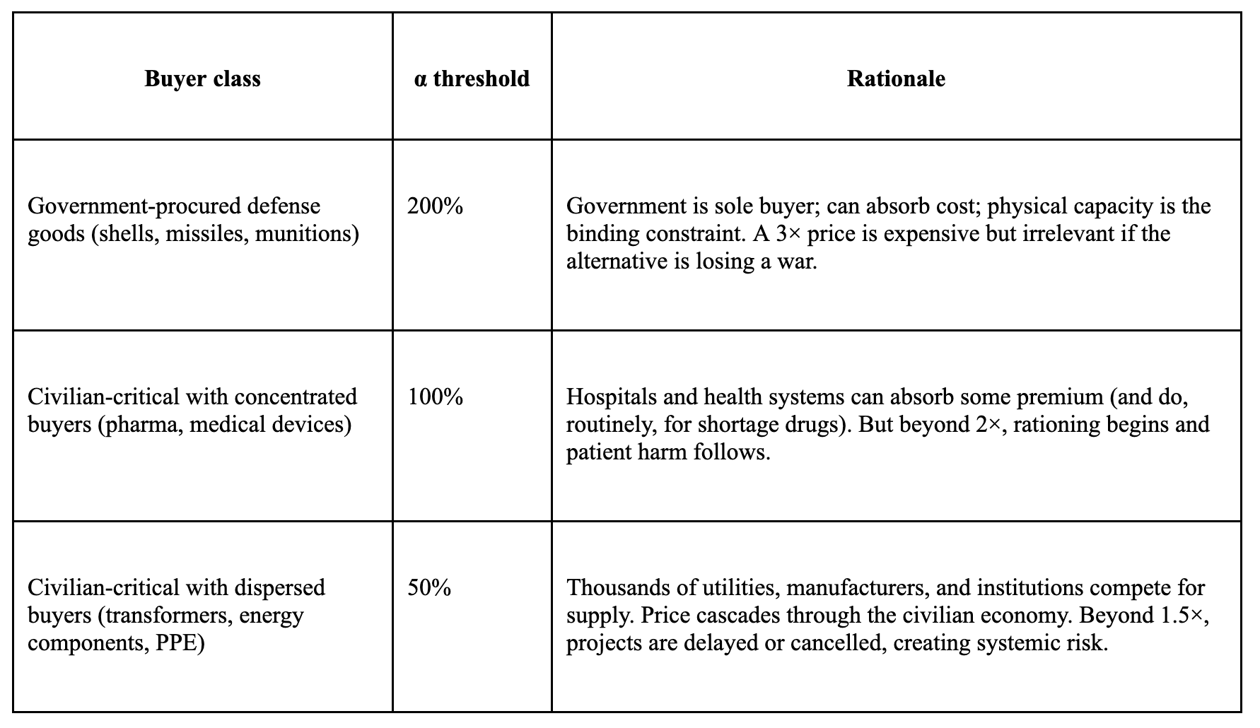
Step 4 - Apply the price penalty: Output surge is worthless if it comes with a price spike that cascades through the civilian economy, but the relevant price threshold depends on who is buying. For government-procured defense goods, the buyer is the federal government, which can and does absorb large cost premiums when the alternative is a capability gap in wartime; the acceptable price increase (α) is set at 200%. For civilian-critical goods with concentrated institutional buyers (hospitals, health systems), α is set at 100%, these buyers can absorb moderate premiums but begin rationing when prices double. For civilian-critical goods with dispersed private buyers (utilities, manufacturers, consumers), α is set at 50%, beyond that, price cascades cause project cancellations, demand destruction, and systemic risk that undermines the purpose of the surge. The formula is:

MEᵢ = β₆ × max(0, 1 − ΔPᵢ/(Pᵢ × α))

This tiered approach reveals three distinct failure modes: sectors where the U.S. cannot physically surge regardless of price (Stinger, gallium), sectors where it can surge but only at prices that destroy downstream economics (N95s, transformers), and sectors where modest surge capacity survives the price screen (munitions, some pharmaceuticals). The policy response differs for each. (These α have been set for illustrative purposes for these calculations and can be changed on a per item basis.)

A tiered α by buyer class:

Step 5 - Aggregate using the harmonic mean: The national ME is the criticality-weighted harmonic mean across the basket:

ME = (Σ wᵢ · (1/MEᵢ))⁻¹

The harmonic mean is needed because the weakest link dominates. An economy that can surge 50% in steel but 0% in rare earth magnets is as vulnerable as its least elastic input. This is the mathematically correct property for a security metric: security is defined by the binding constraint instead of the average.

What the Numbers Reveal

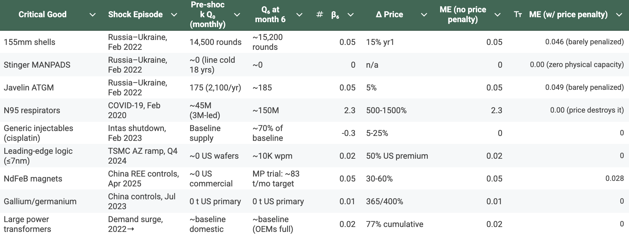
The tables above present ME estimates for nine critical goods, each grounded in a specific historical demand-shock episode with publicly verifiable production data. Full sourcing and methodology are in the Appendix.

Table Details: β₆ is the realized share by which monthly output rose between the start of the historical demand-shock episode and six months later, computed from publicly reported production rates. Sources: Defense One; U.S. Army PEO Ammunition; Lockheed Martin and RTX corporate disclosures; FDA CY2024 Report to Congress; USGS Mineral Commodity Summaries 2025; Wood Mackenzie Q2 2025 Transformer Supply Chain Report; Swedish National China Centre 2025 review of Argus / Fastmarkets / China Customs data; TSMC corporate disclosures.

Four sectors: Stinger (ME = 0, line cold for 20 years), gallium/germanium (ME = 0.01, no primary production), leading-edge logic (ME = 0.02, no surge mechanism in a 3-to-5-year fab cycle), and generic injectables (β₆ = −0.30, supply contracted after the Intas shutdown), have surge capacity at or below zero and are excluded from the harmonic mean. They represent binding constraints requiring distinct policy responses, as described below.

The remaining five sectors produce an aggregate ME of 0.045, meaning the U.S. can scale output by less than 5% within six months even in the sectors where some capacity exists. The 0.50 target remains distant by more than an order of magnitude. Even the N95 success story (β₆ ≈ 2.30, the only genuine surge in the basket) does almost nothing to lift the aggregate because the harmonic mean is dominated by the weakest links.

The price penalty column adds nuance: The relevant threshold depends on who is buying: 200% for government-procured defense goods (the Army will pay 3× per shell if shells exist to buy), 100% for civilian goods with concentrated institutional buyers like hospitals, and 50% for goods with dispersed private buyers like utilities and manufacturers, where price cascades cause project cancellations and systemic risk. Applying these tiered thresholds reveals three distinct failure modes detailed below.

Policy Implications:

America cannot physically surge, price irrelevant: Stingers, gallium, germanium, leading-edge semiconductors, and generic injectables have ME at or near zero regardless of price tolerance. For munitions and minerals, the binding constraint is industrial capacity. For generics, the constraint is structural: concentrated manufacturing, thin margins, and 85% foreign API sourcing mean the system contracts when a major supplier fails instead of surging to compensate. Policy response: DPA Title III investments, second-source qualification, stockpiling, and (for pharmaceuticals) reforming the reimbursement incentives that make domestic API production uneconomic.

America can physically surge but price destroys downstream: N95 respirators and power transformers show positive physical β₆ but zero price-penalized ME. When N95 prices went to 10× list, hospitals rationed and reused them. When transformer prices rose 77%, utilities delayed grid projects. Policy response: strategic reserves sized to bridge the spike, demand-side rationing authorities, pre-negotiated surge pricing contracts.

America can modestly surge at manageable prices: 155mm shells, Javelins, and some generics retain small but real price-adjusted ME. These are the sectors closest to functioning, where marginal investment in warm standby lines and pre-qualified second sources has the highest payoff per dollar.

The target (ME above 0.50) means the U.S. can scale output of critical goods by 50% within 180 days at prices sustainable for the relevant buyer class. This creates accountability for the unglamorous work that actually moves the needle: pre-qualifying backup suppliers, training machinist pipelines, maintaining warm production lines, and positioning strategic stockpiles.

Institutional Design: Making the Numbers Real

Publishing body: The natural home is a new Office of Economic Security Analytics modeled on the analytical independence of the Bureau of Labor Statistics, civil-service economists and supply-chain analysts whose published numbers cannot be edited for political convenience. The 2025 CFR Task Force on U.S. Economic Security recommended dedicated institutional capacity for exactly this function.

The Department of Commerce is also an obvious home (BIS already runs the export-control list, ITA runs trade defense), but it is also a department whose recent track record on industrial policy execution (from the slow CHIPS Act disbursement timeline to the politicized handling of entity-list decisions) gives many people pause. Two alternatives for consideration: (1) a federally chartered nonprofit on the model of MITRE or IDA, contracted by Commerce but operationally insulated; or (2) a joint office reporting to both Commerce and the Director of National Intelligence, on the model of the National Counterintelligence and Security Center. The institutional choice matters less than the principle: the office must have genuine analytical independence and a publication cadence that cannot be halted by an incoming administration that finds the numbers inconvenient.

Publication cadence: Quarterly CEI% dashboard with sector and adversary decomposition, plus a top-10 chokepoint node list and watchlist. Annual ME assessment with sector-level scores, historical backtesting, and explicit policy recommendations for the lowest-ME sectors.

Policy triggers: When CEI% for any single chokepoint exceeds a threshold (when any individual adversary-controlled node puts more than 0.5% of GDP at risk) an automatic interagency review is triggered with a mandatory 90-day action plan. When ME for any critical-basket sector falls below 0.15 (when surge capacity is essentially nonexistent) the same trigger fires.

The Toolkit: What “Action” Actually Looks Like

The Federal Reserve’s dual mandate works because it comes with instruments that move markets within hours. CEI% and ME need their own toolkit: narrower than monetary policy, but real. Five categories of instrument should be linked to the metric:

1. Strategic stockpiling at scale: The Defense Logistics Agency’s National Defense Stockpile is currently funded at roughly $1 billion per year and holds materials worth a fraction of one percent of GDP. When CEI% on a single chokepoint exceeds the 0.5%-of-GDP trigger, the stockpile authority should be empowered to acquire forward inventory equal to 12 months of U.S. consumption of that chokepoint input within 180 days, funded from a standing appropriation that does not require fresh congressional action. This is the equivalent of the Fed’s open-market desk (fast, rule-bound, and large).

2. Defense Production Act Title III investments: DPA Title III already permits direct equity investments and loan guarantees to expand domestic production of critical inputs. When ME for a critical-basket sector falls below 0.15, a DPA Title III action plan should be required within 90 days, with a binding obligation to obligate funds within 180 days. The MP Materials–DOD partnership (which committed to scaling U.S. rare earth magnet capacity from near-zero to an estimated 10,000 metric tons annually by 2028) is the model.

3. Allied-sourcing fast-track: Most resilience gains come from diversification to allies, not reshoring (the OECD 2025 Supply Chain Resilience Review is explicit on this). The dashboard should trigger automatic Section 232 exemptions, USMCA fast-track designation, and AUKUS-style defense procurement carve-outs for inputs sourced from a defined ally bloc when CEI% on the input exceeds the trigger.

4. Demand-side authorities: Drawing on the demand-elasticity insight above, the toolkit should include the authority to suspend non-essential federal procurement of a chokepoint input during a designated crisis (analogous to Cold War priority-rating systems), and to issue voluntary efficiency standards that reduce private-sector demand without triggering an outright price-control regime.

5. Targeted second-source qualification grants: The single most effective cheap intervention is paying the qualification cost for a backup supplier, whether for a missile component or a generic API, so that switching time falls from 18 months to 90 days. The metric should trigger automatic FDA, DOD, and DOE qualification-grant authority for second sources in any critical-basket sector with ME below 0.15.

The analogy to the Fed is imperfect, as there is no “interest rate of economic security”, but the principle holds: a metric without a policy lever is a thermometer in a room with no thermostat. The five instruments above are the thermostat.

What These Metrics Do Not Directly Measure

A qualification on technological leadership. CEI% and ME do not directly measure innovation as a headline metric, but they should not be read as endorsing import substitution at any quality cost. A surge to 30% domestic production of a leading-edge chip at two-generation-old quality is worse than a continued reliance on a single Taiwanese supplier, because the resulting domestic ecosystem cannot actually run the modern applications that economic security is trying to protect. Two guardrails follow:

First, the ME basket should be defined at the relevant performance specification, not at the generic product class: “sub-7nm logic” rather than “semiconductors,” “GaN-on-SiC RF amplifiers above 100 W” rather than “power electronics.” Output that does not meet the relevant spec does not count toward the surge.

Second, when a product class has a specification frontier moving faster than domestic capability can match, the dashboard should flag the gap and refer the question to the existing technology-policy apparatus (CHIPS R&D, DARPA, DOE national labs) instead of pretending the ME framework can resolve it. The dual mandate is necessary but not sufficient, and that’s the point of having a separate technology-leadership policy track that runs alongside it.

Innovation metrics (patent counts, R&D spending, venture capital flows) belong in technology policy, which has its own institutional apparatus and its own billions of annual budget. Conflating economic security with technological leadership allows every dollar justified as “security” to flow toward glamorous frontier research over the unglamorous work of qualifying backup suppliers, training machinists, pre-positioning stockpiles, and maintaining warm production lines.

By limiting the mandate to dependencies (CEI%) and production capacity (ME), these metrics force policy attention onto the industrial base that actually makes things: the layer where the United States is most visibly failing. Examples: The Stinger missile production line was closed. The Army hadn’t bought a Stinger in 18 years. The U.S. hadn’t manufactured its own TNT since 1986. These are production and industrial base failures. CEI% and ME are designed to ensure they never happen again, or at minimum, to ensure that when they do happen, there is a published number that holds policymakers accountable.

While the Fed’s dual mandate did not “solve macroeconomics,” it gave policymakers a common language, a set of targets, and a transparent scorecard. Economic security will benefit from this outlined scorecard with benchmarks like CEI% below 2% of GDP and Mobilization Elasticity above 0.50.

Appendix A: ME Calculation Methodology and Sources

For each critical good i, ME is estimated from a specific historical demand-shock episode. The actual production rate at the start of the shock (Q₀) and six months later (Q₆) are observed, then:

β₆ = (Q₆ − Q₀) / Q₀

This is a direct empirical measure which makes each estimate transparent and replicable, but also specific to the historical episode used. Where the historical baseline is zero, β₆ is reported as zero. Two ME values are reported: ME (physical), which is β₆ alone, and ME (price-adjusted), which applies the tiered price-penalty formula from the main text. The acceptable price threshold (α) varies by buyer class: 200% for government-procured defense goods, 100% for civilian goods with concentrated institutional buyers (hospitals), and 50% for civilian goods with dispersed private buyers (utilities, manufacturers).

A note on zero-baseline sectors. For three sectors (leading-edge logic, NdFeB magnets, gallium/germanium), the pre-shock U.S. production baseline was effectively zero, making the standard β₆ formula undefined (division by zero). For these sectors, ME is estimated as the share of U.S. demand that new or trial domestic capacity could serve within six months of the relevant shock, a related but distinct measure that captures the same policy question: how much can the U.S. produce when it needs to? For one sector (generic injectables), β₆ is negative because the system contracted instead of surging; ME is reported as zero.

155mm artillery shells

α = 200% (defense)

Q₀ = 14,500 rounds/month, the pre-war rate confirmed by Maj. Gen. John Reim (Joint PEO Armaments and Ammunition), reported by Defense One (June 2025) and at a CSIS event (February 2024). Q₆ ≈ 15,200 rounds/month (August 2022): supplemental funding flowed in mid-to-late 2022, but new propellant and TNT lines did not come online until 2024–25. Production reached 28,000/month by October 2023 and 40,000/month by September 2024, where it plateaued through mid-2025, roughly 30 months to roughly triple. The Army’s target of 100,000/month by October 2025 was repeatedly missed and pushed to mid-2026.

Binding constraints were physical: the U.S. hadn’t manufactured TNT since 1986, propellant production depended on imports from Poland, France, Czech Republic, Korea, and Canada, and qualified workers had to be trained from scratch. A $435 million domestic TNT contract (Repkon USA, Graham, Kentucky) was awarded in November 2024.

Price impact: ~+15% unit cost in year one. Well within the 200% defense threshold.

β₆ ≈ 0.05. ME (physical) = 0.05. ME (price-adjusted) ≈ 0.046.

Stinger MANPADS

α = 200% (defense)

Q₀ ≈ 0/month: RTX had not built new Stingers in roughly 20 years. The Pentagon awarded a $624.6 million contract for 1,300 missiles in May 2022. Q₆ ≈ 0/month: then-CEO Greg Hayes told investors in April 2022 that Raytheon could not ramp production until 2023 because the missile contained obsolete components requiring redesign. Wes Kremer (former Raytheon president) estimated 30 months from contract to first units, retired employees were drafted to teach current staff how to build the missile.

By 2024, Raytheon was ramping to 60 Stingers/month (FlightGlobal). A $700 million NATO contract (2024) added 940 missiles for Germany, Italy, and the Netherlands. A Raytheon spokesperson told Breaking Defense in August 2025 the company is “doubling Stinger production capacity over the next five years.”

Price impact: irrelevant: zero output means no market price for surge units.

β₆ ≈ 0.00. ME = 0.00.

Javelin ATGMs

α = 200% (defense)

Q₀ ≈ 175/month (2,100/year), per Lockheed Martin’s media kit and February 2024 corporate update. Q₆ ≈ 180–200/month: modest overtime ramp, no meaningful capacity addition. The ramp from 2,100 to 2,400/year (14% increase) took until 2024. The further ramp to 3,960/year requires 14 new test stations in Troy, Alabama and 8 in Ocala, Florida, targeting late 2026, a 50%+ expansion taking approximately four years. On August 29, 2024, the Army awarded the JJV a $1.3 billion contract, the largest single-year Javelin contract to date.

Price impact: ~+5%. Negligible against the 200% threshold.

β₆ ≈ 0.05. ME (physical) = 0.05. ME (price-adjusted) ≈ 0.049.

N95 respirators

α = 50% (dispersed civilian buyers)

Q₀ ≈ 45 million/month domestically (3M-dominated). Q₆ ≈ 150 million/month by August 2020: 3M roughly tripled output, Honeywell stood up new lines, and dozens of new entrants added capacity under DPA Title III orders. β₆ ≈ 2.30, by far the highest in the basket and the only case of genuine surge capacity.

But spot prices rose 5× to 15× depending on grade and channel; hospitals reported paying 10× list. This far exceeds the 50% threshold for dispersed civilian buyers. The physical surge was real; the economic surge was fictitious.

β₆ ≈ 2.30. ME (physical) = 2.30. ME (price-adjusted) = 0.00.

Generic sterile injectables (cisplatin/carboplatin)

α = 100% (concentrated institutional buyers - hospitals)

Intas Pharmaceuticals (Accord Healthcare) facility shutdown after FDA inspection findings, February 2023. Intas supplied roughly 50% of U.S. cisplatin. Q₆ ≈ 70% of baseline: emergency imports from Qilu (China) and 503B compounders restored partial supply by mid-2023, but the Intas facility remained below normal through Q3.

Structural context: per the FDA’s CY2024 Report to Congress, 1,459 potential shortage situations were reported by 151 manufacturers that year. Manufacturers operate at 80%+ capacity with thin margins; 85% of APIs come from foreign facilities (ASPE January 2025 brief); 40% of generic drug markets have a single manufacturer; roughly 272 active shortages tracked by ASHP as of mid-2025.

Price impact: cisplatin rose ~25%, within the 100% hospital-buyer threshold.

β₆ ≈ −0.30: the system contracted instead of surging, with output falling to roughly 70% of baseline by month six. This is a structural fragility. ME (physical) = 0.00. ME (price-adjusted) = 0.00.

Leading-edge logic (≤7nm)

α = 50% (dispersed civilian buyers - fabless chip companies)

No historical demand-shock episode exists because there was essentially no U.S. leading-edge logic to surge. TSMC Arizona is the relevant proxy: committed 2020, broke ground 2021, Phase 1 entered N4 production Q4 2024, a four-year construction cycle. Mid-2025 output: ~15,000 wafer-starts/month, ramping toward design capacity of ~24,000 wpm. Global TSMC leading-edge capacity exceeds 150,000 wpm; Arizona is ~10% of that. Phase 2 (3nm) targets H2 2027; Phase 3 (2nm/A16) broke ground April 2025. Total committed investment: $165 billion, the largest FDI in a U.S. greenfield project in history.

There is no physical mechanism by which leading-edge wafer output can surge in 180 days. New fab construction takes three to five years.

Price impact: U.S.-made chips carry a ~50% cost premium over Taiwan-made equivalents, right at the threshold.

ME ≈ 0.02. ME (price-adjusted) ≈ 0.00.

NdFeB rare earth magnets

α = 100% (mixed defense + industrial buyers)

China’s April 2025 export controls on seven categories of rare earth elements and magnets. Q₀ ≈ ~0 commercial U.S. NdFeB magnet production; MP Materials’ Independence facility in Fort Worth was in trial production. Q₆ ≈ ramping toward 1,000 MT/year (≈83 MT/month) against U.S. demand of 10,000–15,000 MT/year.

DOD and MP Materials announced a public-private partnership to build a “10X” facility (additional 7,000 MT capacity, plus Independence expansion to 3,000 MT), targeting 10,000 MT total by commissioning in 2028.

Price impact: NdFeB magnet prices rose ~45%, within the 100% threshold but close to halving the score.

β₆ ≈ 0.05 vs. U.S. demand. ME (physical) = 0.05. ME (price-adjusted) ≈ 0.028.

Gallium and germanium (primary)

α = 100% (mixed defense + semiconductor buyers)

China’s July 2023 export-licensing requirement reduced unwrought gallium exports by 66% in the post-control period (Argus / China Customs data, per Stimson Center analysis, April 2025). Q₀ = 0 metric tons of U.S. primary low-purity gallium. Per USGS Mineral Commodity Summaries 2025: China accounts for 99% of worldwide primary production; “at least one company is exploring the feasibility of producing domestic primary gallium.” Q₆ = still zero.

Some recycling and stockpile drawdown softened the impact. In November 2025, China temporarily suspended its export ban through November 2026. USGS estimated a total ban could cost the U.S. economy approximately $3.4 billion in output.

Price impact: gallium +365%, germanium +400%, antimony +437% (Swedish National China Centre, December 2025, reviewing Argus and Fastmarkets data). Far above any reasonable α.

β₆ ≈ 0.01 (reflecting marginal secondary recovery and stockpile drawdown, not primary production surge). ME (physical) = 0.01. ME (price-adjusted) = 0.00

Large power transformers

α = 50% (dispersed civilian buyers - utilities)

Post-2022 demand surge driven by data centers, electrification, and aging infrastructure. Wood Mackenzie estimates power transformer demand up 116% since 2019; GSU demand up 274%. Lead times: 128 weeks (2.5 years) for power transformers, 144 weeks for GSUs, per Wood Mackenzie Q2 2025 survey. Imports account for an estimated 80% of U.S. power transformer supply in 2025. More than half of the roughly 60–80 million U.S. distribution transformers in service are beyond their expected life.

Domestic capacity expansions since 2023 total ~$1.8 billion (Eaton in South Carolina by 2027; Siemens Energy in North Carolina early 2027; Hitachi Energy in Virginia and Pennsylvania), none on a six-month timescale. Supply deficit: 30% for power transformers, 10% for distribution transformers in 2025.

Price impact: +77% cumulative since 2019; utilities report paying 4–6× pre-2022 costs. Well above the 50% threshold.

β₆ ≈ 0.02, reflecting marginal import increases but no demonstrated domestic production surge, all major OEMs report full order books with no available production slots. ME (physical) = 0.02. ME (price-adjusted) = 0.00.